Introducing Skorecard for building better logistic regression models
skorecard is an open source python package that provides scikit-learn compatible tools for bucketing categorical and numerical features and building traditional credit risk acceptance models (scorecards) on top of them. These tools have applications outside of the context of scorecards and this blogpost will show you how to use them to potentially improve your own machine learning models.
Bucketing features is a great idea
Bucketing is a common technique to discretize the values of a continuous or categorical variable into numeric bins. It is also known as discretisation, quantization, partitioning, binning, grouping or encoding. It's a powerful technique that can help reduce model complexity, speed up model training, and help increase understanding of non-linear dependencies between a variable and a given target. Bucketing and then one-hot encoding features can introduce non-linearity to linear models. Even modern algorithms use bucketing, for example LightGBM that buckets continuous feature values into discrete bins and uses them to construct feature histograms during training (paper). Bucketing is also widely used in credit risk modelling (where linear models are often used) as an essential tool to help differentiate between high-risk and low-risk clients.
Bucketing is a great idea to improve the quality of your features, especially if you are limited to linear models. With 'the right features a linear model can become a beast', as argued in Staying competitive with linear models. A good example is the explainable boosting machine (EBM) algorithm developed by Microsoft. It uses a novel way to detect interaction terms to breathe new life into generalized additive models, with performance comparable to state-of-the-art techniques like XGBoost (paper).
Bucketing can be done univariately and can be unsupervised or supervised, and done on categorical or numerical values. Some examples:
- Unsupervised & numerical:
sklearn.preprocessing.KBinsDiscretizerthat bins a continuous feature intokbins using different strategies. - Unsupervised & categorical:
sklearn.preprocessing.OrdinalEncoderthat encodes each unique value of a categorical feature into an ordinal integer. - Supervised & numerical:
skorecard.bucketers.DecisionTreeBucketertrains a DecisionTreeClassifier on a single feature and uses the tree output to determine the bucket boundaries - Supervised & categorical:
skorecard.bucketers.OrdinalCategoricalBucketerwill create an ordinal bucket number sorted by the mean of the target per unique value, where the most common values will have a lower bucket number.
Bucketing in skorecard
skorecard offers a range of so-called bucketers that support pandas dataframes. There is support for different strategies to treat missing values as well as the possibility to define 'specials': certain values you would like to ensure get put into a separate bucket. And there are tools to inspect the resulting bucketing. Here's a simple example:
import pandas as pd
from skorecard.bucketers import EqualWidthBucketer

df = pd.DataFrame({'feature1': range(10) })
bucketer = EqualWidthBucketer(n_bins=5)
df = bucketer.fit_transform(df)
bucketer.bucket_table('feature1')
#>    bucket        label  Count  Count (%)
#> 0      -1      Missing    0.0        0.0
#> 1       0  (-inf, 1.8]    2.0       20.0
#> 2       1   (1.8, 3.6]    2.0       20.0
#> 3       2   (3.6, 5.4]    2.0       20.0
#> 4       3   (5.4, 7.2]    2.0       20.0
#> 5       4   (7.2, inf]    2.0       20.0
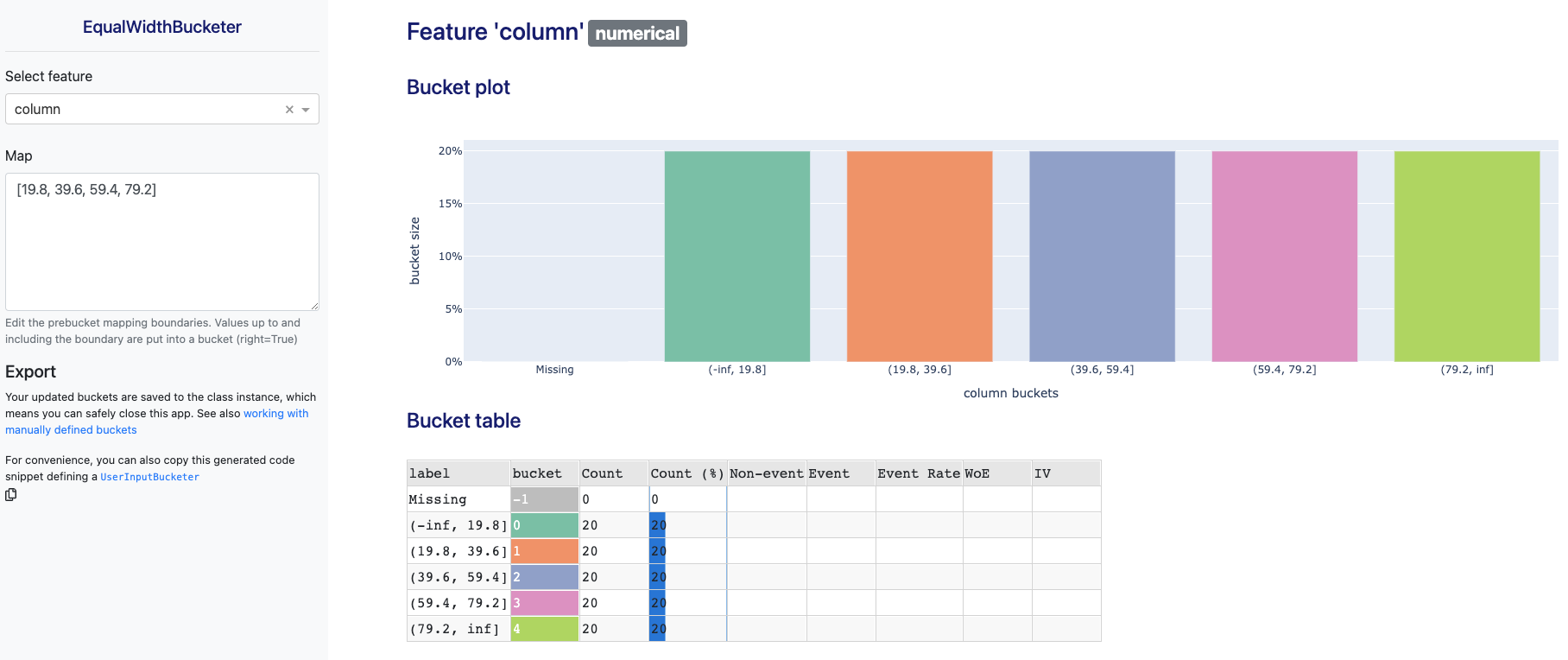
When using bucketing in an actual use case like credit decision modelling, there are often all kinds of constraints that you would like to impose, like the minimal relative size of each bucket or monotonicity in the target rate per bucket. It's also common to discuss and incorporate domain expert knowledge into the bucketing of features. This manual 'fine tuning' of the bucketing is an interplay between art and science. skorecard offers support for bucketing under constraints (see OptimalBucketer) as well as a novel .fit_interactive() method that starts a dash webapp in your notebook or browser to interactively explore and edit buckets. Expanding on the example above, we can also do:
Weight of Evidence encoding can improve performance
After bucketing, Weight of Evidence (WoE) encoding can help to improve binary logistic regression models. WoE encoding is a supervised transformation replaces each bucket (category) in a feature with their corresponding weight of evidence. You can find the weight of evidence for a bucket by taking the natural logarithm of the ratio of goods (ones) over the ratio of bads (zeros). So, if a certain bucket has 60% ones and 40% bads, the WoE would be ln(0.6/0.4) = 0.405. More formally:
The higher the WoE, the higher the probability of observing Y=1. If the WoE for an observation is positive then the probability is above average, if it's negative, it is below average. Using WoE encoding after bucketing means you can build models that are robust to outliers and missing values (which are bucketed separately). The natural logarithm helps to compare transformed features by creating the same scale and it helps to build a strict linear (monotonic) relationship with log odds. When combined with a logistic regression this method has also been called the 'semi-naive bayes classifier' because of it's close ties with naive bayes (this blogpost for more details).
A downside of WoE encoding is that you need buckets that have observations with both classes in the training data, otherwise you might encounter a zero division error. That's why skorecard bucketers have a min_bin_size parameter that defaults to 5%. In practice, it means you'll want to bucket features to max ~10-20 buckets. And if you're using cross validation, you need to make sure the bucketing and WoE encoder are part of the model pipeline.
The WoE encoder is quite common and there are many python implementations available online. Instead of implementing another one, skorecard uses scikit-learn contrib's category_encoders.woe.WOEEncoder:
from skorecard import datasets
from category_encoders.woe import WOEEncoder

X, y = datasets.load_uci_credit_card(return_X_y=True)
we = WOEEncoder(cols=list(X.columns))
we.fit_transform(X, y)
skorecard as a stronger baseline model
A good data scientist will start with a stupid model because a good baseline model can tell you if your data has some signal and if your final shiny model actually provides a performance increase worth the additional complexity. You want to apply Occam's razor to machine learning: prefer the simpler model over the complex one if performance is more or less equal. But a big complex model that has spent a lot of compute on hyperparameter tuning will likely outperform a humble quick LogisticRegression model. Before declaring victory, applying some smart auto-bucketing and weight of evidence encoding might offer a more performant and fair comparison. And it's a one-liner in skorecard:
I ran a benchmark using the UCI Adult, Breast Cancer, skorecard UCI creditcard, UCI heart disease and Kaggle Telco customer churn datasets. We compare a LogisticRegression with one hot encoding of categorical columns (lr-ohe), a variant with ordinal encoding of categoricals (lr-ordinal), a typical RandomForest with 100 trees (rf-100), a XGBoost model (xgb) and of course a Skorecard model with default settings.
| dataset_name | model_name | test_score_mean |
|---|---|---|
| telco_churn | lr_ordinal | nan |
| telco_churn | xgb | 0.825 |
| telco_churn | rf-100 | 0.824 |
| telco_churn | lr_ohe | 0.809 |
| telco_churn | skorecard | 0.764 |
| heart | skorecard | 0.911 |
| heart | lr_ohe | 0.895 |
| heart | lr_ordinal | 0.895 |
| heart | rf-100 | 0.89 |
| heart | xgb | 0.851 |
| breast-cancer | skorecard | 0.996 |
| breast-cancer | lr_ohe | 0.994 |
| breast-cancer | lr_ordinal | 0.994 |
| breast-cancer | rf-100 | 0.992 |
| breast-cancer | xgb | 0.992 |
| adult | xgb | 0.927 |
| adult | lr_ohe | 0.906 |
| adult | rf-100 | 0.903 |
| adult | skorecard | 0.888 |
| adult | lr_ordinal | 0.855 |
| UCI-creditcard | skorecard | 0.627 |
| UCI-creditcard | lr_ohe | 0.621 |
| UCI-creditcard | lr_ordinal | 0.621 |
| UCI-creditcard | xgb | 0.596 |
| UCI-creditcard | rf-100 | 0.588 |
Table 1: Benchmarking skorecard with other baseline models. See also benchmark notebook if you want to reproduce the results.
The table shows that Skorecard frequently outperforms LogisticRegression and even more complex algorithms (that haven't been tuned yet), but in line with the no free lunch theorem not always. So while skorecard is a great baseline model, you will always want to use a range of simple models to get a sense of the performance of your final model.
Conclusion
Bucketing features is a powerful technique that can help model performance and improve the interpretability of features. Bucketing in combination with weight of evidence encoding can make a logistic regression model much more powerful. skorecard has bucketing transformers you can use in your own modelling pipelines and a Skorecard() estimator that helps automate the bucketing+woe encoding technique and can be more competitive than LogisticRegression. skorecard is a strong approach that you could consider adding to your baseline models.
In the skorecard documentation there are more interesting features to explore such as support for missing values (tutorial), special values for bucketing (tutorial), a two step bucketing approach (tutorial) and the interactive bucketing app (tutorial).